7-June-2017: PHYS 4A--Physical Pendulum Lab

Eric Chong

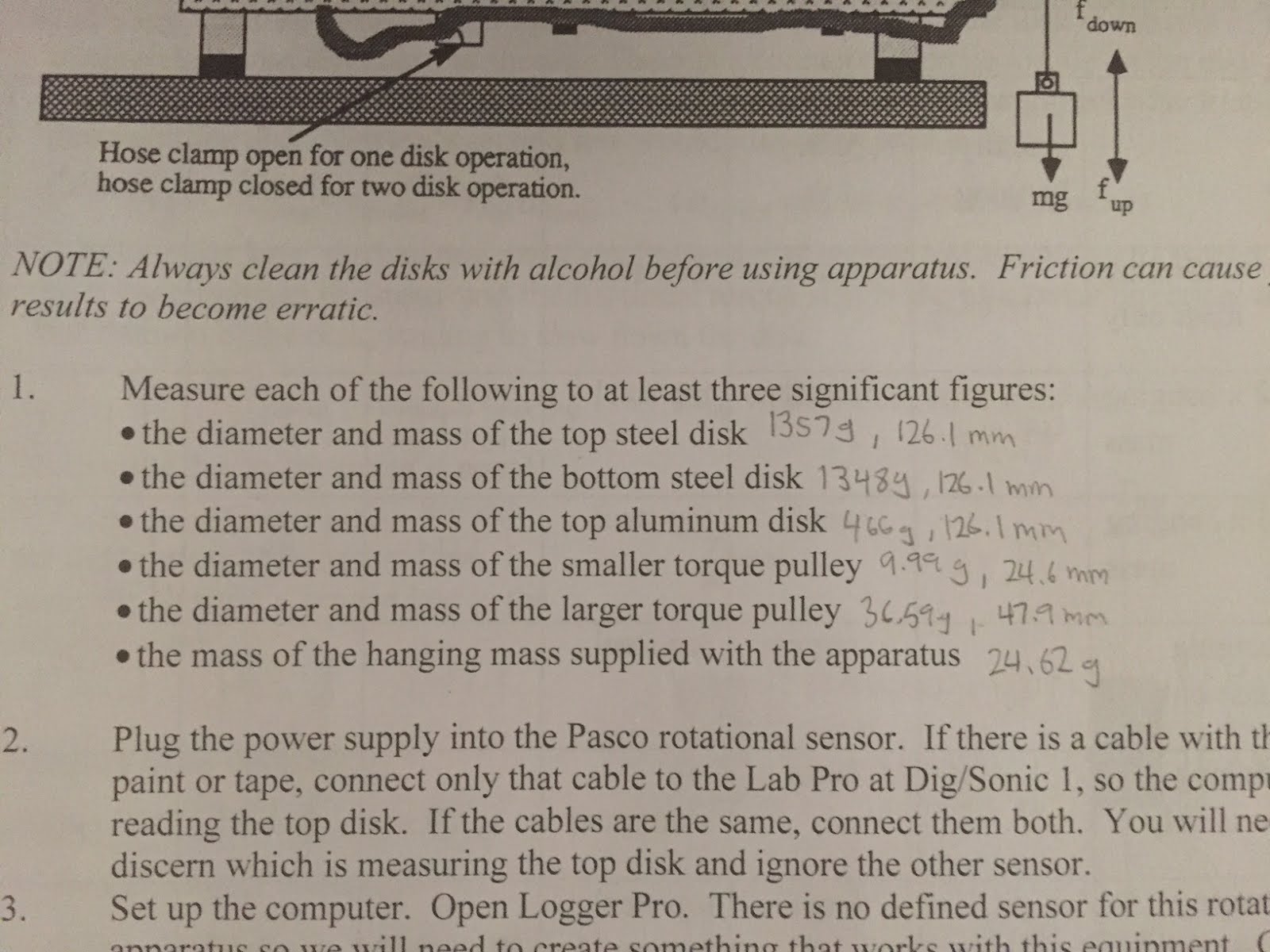
PHYS 4A--Physical Pendulum Lab

Lab Partners: Ben, Nina Song, and Joel Cook

Purpose: Derive expressions for the period of various physical pendulums. Verify your predicted periods by experiment.

Introduction: Objects with mass have a certain moment of inertia that depends on its radius and the place where the pivot is placed. This is essential to finding out the period for physical pendulums. Physical pendulums are rigid bodies mounted on a horizontal axis, so that it can freely oscillate back and forth. The moment of inertia dictates the tendency for the pendulum to move. If there is a higher moment of inertia, the object will have a larger moment of inertia, then the object will have a larger period. If the object has a smaller moment of inertia, then the object will have a smaller period. This is given through the equation alpha = -(mgr/I)theta. This equation is derived from the torque equation, and it will be explained how through the calculations shown in the pictures later, but we solve for the acceleration or angular acceleration because in simple harmonic motions, the acceleration can be used to solve for the period, since the coefficient next to the theta (or position) is the omega. If we take (mgr/I) as omega^2, then we can solve for just omega, and plug that omega into the equation for period, which is T=2pi/omega. This will help us solve for the period. And as expected, the inertia will affect the numerator of the period equation when we plug in omega, so that means that the higher the inertia the larger the period, or the lower the inertia the lower the period. Through this reasoning, calculation, and analysis, we can solve for the periods of the physical pendulums.

Procedure: First, professor had us do a prelab worksheet with questions about a half circle and a triangle, and the work can be seen here:

Generally, we first found the moment of inertia of an object pivoted at one end. And then we found the position of the center of mass and used the parallel axis theorem to find the moment of inertia of the object at the center of mass. After doing so, we can then use the parallel axis theorem again in order to find the moment of inertia of the object at another pivot. This is what we did for both the triangle and the half circle.

Upon doing the lab, we first measured the radius of the half circle, and the base and height of the triangle. With this, we can use those values to solve for the value of the moment of inertia, and then use that to calculate the value of omega, which can be used to solve for the period by dividing 2pi by omega. Here are our calculations with the measured values:

Half Circle:

(Note: the sin(theta) is approximated to a small angle, so we can treat it as just theta)

Triangle:

Our predicted values are 0.708 seconds for the half circle and 0.674 seconds for the triangle.

With these values, we wanted to test the prediction and oscillated the half circle and triangle. We set up LoggerPro and a motion sensor that can detect the period of the oscillation of objects. Here are the setup, graph, and data:

Half Circle:

Triangle:

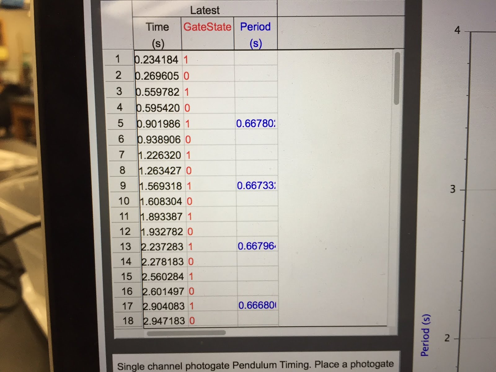
As expected, both periods were around 0.708 and 0.674 seconds for the half circle and triangle, respectively. This means that the calculations were correct, and that the small angle approximation is valid.

Conclusion: The experimental results are very close to what we derived. Based on the calculations, the period of the physical pendulum does not depend on the mass of the pendulum, so even if we added the mass of the paper clip it would not affect the period all that much. The masking tape, however, would be expected to have a bigger effect on the pendulum because the radius would be increased, and therefore increasing the moment of inertia. However, we combated this by making the masking tape relatively thin and small.

Overall, the lab is successful in showing how the moment of inertia of an object can be calculated, how the period can be calculated from solving for the acceleration and taking the omega and dividing 2pi by omega. We were able to set up the experiment and obtain data for the periods of both the half circle and triangle to a relatively small percent error. Some sources of uncertainty could come from the radius of the masking tape, the frictional torque from the pivot, and the dimensions of the half circle and the triangle, since they were not completely flat.

31-May-2017: Lab 19: PHYS 4A Lab--Conservation of Energy/Conservation of angular momentum

Eric Chong

Lab 19: PHYS 4A Lab--Conservation of Energy/Conservation of angular momentum

Lab Partners: Nina Song and Joel Cook

Purpose: To predict and measure how high the clay-stick combination should rise after a collision.

Theory/Introduction: The conservation of angular momentum is very similar to the conservation of momentum. The equation is given in the form of Itotal initial * ωinitial = Itotal final * ωfinal, where I is the moment of inertia, and omega is the angular velocity. Using this idea, we can find the total energy of the system and see what form energy it is converted to, such as from gravitational potential energy to rotational kinetic energy, while also combining it with the concept of conservation of angular momentum if a collision occurs. For this experiment, we will be applying the concepts of conservation of angular momentum for the collision of the meter stick and the clay, and the conservation of energy for the transfer of energy between rotational kinetic energy and gravitational potential energy, in order to find how high the clay-stick combination will rise after the collision.

Procedure: To start, we measured the mass of the meter stick and the clay. Both of their masses turned out to be 146.63 g and 34.54 g respectively. Next, we set up an apparatus that looks like this:

(meter stick has nails sticking out in order to help the clay stick)

Before we commence the experiment, we predicted the height at which the clay-stick combination would rise through calculations. We first used conservation of energy of the stick that is angled at 90 degrees horizontally and made it rotate downwards, gaining rotational kinetic energy, until right before it hits the clay. In doing so, we would also have to use the parallel axis theorem to find the moment of inertia, because the pivot has been shifted to the 10 cm mark of the meter stick. We then used the conservation of angular momentum to calculate the final angular velocity. Finally, we used conservation of energy again, but this time with a new moment of inertia, because the clay sticks onto the stick and contributes some moment of inertia, and the new angular velocity, calculated through the conservation of angular momentum. The variable we need to find is theta, the angle. By finding the angle, we can use the value in order to find how high the clay-stick combination rises. Here is what the calculations look like:

The calculations indicate that the clay-stick combination will rise approximately 30 cm.

We next conducted the experiment. We video captured the motion of the stick rotating and colliding with the clay and rising up to a certain height, and plotted the initial position of the clay and the clay's final height. Here is what we found:

The result is strikingly close to what we predicted. The reason that the value is a bit off is most likely that our plotting skills with LoggerPro are not pixel accurate. Since a centimeter is really small, it is possible that even a pixel on LoggerPro could be a centimeter or a half. Nonetheless, we are more concerned with the overall value and how close it is to what we predicted, and looking at this value of 32.45 cm, we are safe to assume that what we predicted was indeed correct.

Conclusion: This experiment showcases the concepts of conservation of energy with rotational kinetic energy and gravitation potential energy, and the conservation of angular momentum. This lab is meant to help us utilize our skills in order to find certain values at certain times while the stick is in motion. And because of this, this lab has high value for our understanding of physics and engineering skills. Some places of uncertainty may lie in the plotting of the graph in LoggerPro, some loss of energy while the meter stick is in motion (most likely due to the fact that there is drag force or friction in between the pivot point and the meter stick), or maybe even the possibility that the meter stick is not exactly 90 degrees when it started (it could have easily been 91 or 89 degrees). Overall, we are safe to say that, due to our predictions being really close to the actual experimental value, the experiment is a success!

22-May-2017: Lab 17: PHYSICCS 4A LAB--Finding the moment of inertia of a uniform triangle.

Eric Chong

Lab 17: PHYSICS 4A LAB--Finding the moment of inertia of a uniform triangle.

Lab Partners: Nina Song and Joel Cook

Purpose: To determine the moment of inertia of a right triangular thin plate around its center of mass, for two perpendicular orientations of the triangle.

Theory/Introduction: For this lab, we will be exercising the concept of the summation of moments of inertia in order to calculate the moment of inertia of the entire system. This time, we will be using the reverse, by taking the moment of inertia of the system in order to find the moment of inertia of an individual triangle plate. We will be using this theory and another approach, the approach of using the parallel axis theorem to calculate the moment of inertia of the triangle at its center of mass, and comparing the two in order to validate our results. By doing this, we can confirm that the two concepts are equally valid for calculating the moment of inertia of the triangle.

Procedure: We start by using the same setup as the Rotational acceleration lab. Here is what the apparatus looks like:

We use this apparatus and LoggerPro in order to measure the angular acceleration of the apparatus. This is so we can use the equation that we developed in a previous lab. The equation will be shown in the calculation. We first measured the angular acceleration without the triangle. Before we launched the apparatus, we measured the mass of the hanging mass, which turns out to be 25 grams or 0.025 kg, and the radius of the pulley, which turns out to be 0.0248 m. We did this for the calculations portion. We then launched the apparatus and measured its angular acceleration by looking at the slope of the velocity vs. time graph. Here is what the graph looks like:

Here we can see that the angular accelerations going up and down are different. We combat this by taking the average of the two. Next, we calculated the moment of inertia of the apparatus by doing this calculation:

(Note: m is the hanging mass, r is the radius of the pulley, and the denominator is the average of the angular acceleration going up and down.)

We found the moment of inertia of the apparatus alone to be 0.000965387 kg*m^2. With this we can then calculate the moment of inertia of the triangle by doing the same procedure we did, but instead placing the triangle on the apparatus in an upright orientation, calculating the moment of inertia with the same equation, and then subtracting the result with the moment of inertia of the apparatus alone. Here is the apparatus with the upright triangle looks like:

Here is what the graph on LoggerPro looks like after we launched the apparatus:

After finding the angular accelerations and taking the average, we then performed the same calculation for this apparatus-triangle system. Here is the calculation:

The last part of the calculation is simply taking the difference between the moment of inertia of the apparatus-triangle system, which is 0.001239333 kg*m^2, with the moment of inertia of the apparatus alone. The moment of inertia of the upright triangle turns out to be 0.000273946 kg*m^2.

For the next part, we turned the triangle sideways, so that its longer side becomes the base. Here is what it looks like:

We performed the same procedure as before, so here is the graph with the angular acceleration:

Here is the calculation:

The moment of inertia of the sideways triangle turns out to be 0.000588837 kg*m^2.

We now want to confirm our calculations by using the other approach, the approach using the parallel axis theorem in order to find the center of mass moment of inertia of the triangles. The results should be the same or close. Here is the derivation for the moment of inertia of the triangles at the center of mass:

We found that the moment of inertia at the triangle's center of mass is (1/18)MB^2, with M being the mass of the triangle, and B being the base of the triangle. With this, we measured the mass of the triangle, which turns out to be 0.456 kg. For the shorter base of the triangle, we found that the length is 98.2 mm or 0.0982 m. For the longer base of the triangle, we found that the length is 149.1 mm or 0.1491 m. With these measurements, we can finally perform the calculations. Here are the calculations:

Looking at these calculations, it seems that the two types of approaches validate each other. This means that both ways are valid ways of finding the moment of inertia of the triangle.

Conclusion: The lab is a success in that we were able to find the moment of inertia of the upright and sideways triangle using two different approaches. One way is the use of the angular acceleration and measuring the mass of the hanging mass and the radius of the pulley and using the desired equation that we used in a previous lab. The other way is to use the moment of inertia of the triangle at its center of mass, and plugging in the mass of the triangle and their respective bases. Both approaches confirm that the moments of inertia of the upright and sideways triangle are close to the calculations. Some sources of uncertainty could come from our measurements of mass, length, base, radius, etc. Another source of uncertainty could come from the pulley, as it is not an ideal pulley, as seen in the differing angular accelerations going up and down. Overall, this lab is successful and we were able to learn that both ways of calculating the moment of inertia of the triangles are valid.

22-May-2017: LAB 18: A LAB PROBLEM--MOMENT OF INERTIA and FRICTIONAL TORQUE

Eric Chong

LAB 18: A LAB PROBLEM--MOMENT OF INERTIA and FRICTIONAL TORQUE

Lab Partners: Nina Song and Joel Cook

Purpose: The goal of this lab is to measure the time it takes for a cart tied to a string connected to a large metal disk on a central shaft, by measuring and calculating the total moment of inertia and the acceleration the cart will experience.

Theory/Introduction: The moment of inertia is different for each individual objects. However, the moment of inertia of a system can be calculated through the sum of the individual moments of inertia of the individual objects. In the net torque equation, the net torque is equal to inertia times the angular acceleration. We can find the angular acceleration through video analysis. With this, it is possible to calculate the net torque the system has, and by using the relationship with the net force equation, it is possible to solve for the acceleration of the cart.

Procedure: We first start this lab by measuring the radius and height of each cylinder (2 small and 1 large) of the apparatus that looks like this:

After measuring the radius and height of each cylinder, we started calculating the volume of each and totaling the volume. We do this because the cylinders have uniform mass, meaning that the volume is proportional to the mass. If we can get the percent volume of each individual cylinder, we can figure out their individual masses, given the total mass of the apparatus. And once we have their masses, we can calculate for their individual moments of inertia. And finally, we can get the total moment of inertia by adding each of their moments of inertia together. Here are the measurements and calculations we did:

(To make calculations easier, we assumed that the two smaller cylinders have the same radii and height.)

Our total moment of inertia came out to be 0.0199 kg*m^2, which is what we expected based on what the professor said. Next, we started doing video analysis by recording the spin of the apparatus, in order to measure its angular acceleration. We used LoggerPro for this part and plotted points on the rim of the big cylinder as it was spinning. Through this, we can analyze the angular acceleration by looking at the slope of the angular velocity vs. time graph. We derived the angular velocity equation in LoggerPro by inputting the equation, omega = (Vtangential)/R, where omega is the angular velocity. Here is what the graphs looks like:

(This is the position vs. time graph)

(Here is the omega vs. time graph)

The angular acceleration, by looking at the slope, is -0.1903 rad/s^2. We also quickly measured the angle of the slope the cart is traveling on, which turns out to be 40 degrees. With this, we now have all of the variables needed to calculate the acceleration of the cart. We set up two equations. One is the net force equation, and the other is the net torque equation. Through manipulation, we are able to solve for the acceleration the cart experiences, and in turn the time it takes for the cart to travel 1 meter, the length of the slope. Here is the calculation:

Our calculation shows that the time it takes is approximately 7.0515 seconds. We then ran 5 trials to test the calculation. Here is what we got:

It is seen that all of the trials are above the calculated value, which is a sign for a sort of systematic error. Perhaps the pulley is not as ideal as we thought, and may have contributed a slight frictional torque on the system. Or perhaps the slope that the cart was traversing on is not entirely frictionless. Or maybe that the way the string is strung on the cylinder is a contributing factor to the slight error in the measurements, in that maybe the tension is not quite equal to mgsin(theta), because as the cart was going down, the tension might be changing as the cart is speeding up.

Conclusion: The lab is successful, in that even though our data is not quite as what we expected, we were able to maintain an error within 5%. This still confirms that our method is still largely correct, and that perhaps we need some slight adjustments with the pulley, the slope, or the cart in order to provide better data closer to the calculations. Some sources of uncertainty may have come from the pulley itself, since frictional torque is a possibility, the slope itself, since it could have had friction on the cart, or the string, since I suspect that there might be a sort of changing tension as the cart was speeding up. Overall, the lab showcases how to calculate the moments of inertia of each individual piece, and adding them up in order to find the total moment of inertia, how to find the angular acceleration through video analysis, and how both the net force and net torque equations are related and can be used to find the acceleration of the cart.

8-May, 15-May-2017: Lab 16: Angular acceleration

Eric Chong

Lab 16: Angular acceleration

Lab Partners: Nina Song and Joel Cook

Purpose: Observe the effects of changing the hanging mass, the radius at which the hanging mass exerts torque, and the rotating mass on the angular acceleration.

Theory/Introduction: The angular acceleration of a disk is affected by the radius of the disk, the rotating mass, and the intensity of the torque exerted at a certain radius. We want to experiment with how each of these factors affect the angular acceleration. We can test the effect of changing the intensity of the force exerted at a certain radius by attaching a string perpendicular to the disk's radius and changing the hanging mass's mass in order to increase or decrease the torque exerted on the disk. We can test the effect of changing the radius by changing the size of the pulley that is made of the same material.  We can also test the effect of changing rotating mass itself by changing the material of the disk with an aluminum disk and a steel disk; this change will affect the inertia. By doing this experiment, we can determine how angular acceleration is affected when these factors are incorporated, and ultimately find through calculations how this all comes together. We can also determine certain relationships at the start by looking at the equation, torque = I*alpha, where I is the moment of inertia, and alpha is the angular acceleration. This relationship will be discussed later in the lab.

Procedure: Part 1) For this Part of the experiment, we just want to see how the factors mentioned in the introduction affect the angular acceleration of a rotating mass. We start by setting up the apparatus like so:

The hanging mass is connected to a string, which is connected to the rotating mass. An air is used to reduce friction. The apparatus is also connected to LoggerPro in a laptop, so we can measure the angular velocity of the rotating mass, as we observe the factors affecting the angular acceleration. We first observed the effects of the change in the mass of the hanging mass on the angular acceleration, and then the effects of changing the radius, and finally the effects of changing the rotating mass. For the hands-on measurements, here is the data:



Here is what we got on LoggerPro when we changed the hanging mass by doubling and tripling it, the radius of the pulley by doubling its size, and the disk itself by changing it from "top steel" to "top aluminum" and "top steel + bottom steel," in that order:

We can look at the angular acceleration by looking at the slopes of the velocity vs. time graphs while the hanging mass was going up and down. Upon observation, the angular acceleration seems to be changing while it is going up and down. We hypothesize that the reason the angular accelerations are different while going up and down is that there is a sort of frictional torque affecting the angular acceleration. To take this into account, we evaluated the angular acceleration by taking the average of the values while the hanging mass is going up and down. Here is a data table of all of the changes we made to the apparatus and its corresponding angular acceleration values:

It seems that by doubling the hanging mass, we also doubled the angular acceleration, and when we tripled the mass of the hanging mass, we tripled the angular acceleration. Furthermore, when we doubled the radius of the torque pulley, we also doubled the angular acceleration. We can also determine through the analysis of the torque = I*alpha equation that it is likely that changing the inertia will have an inverse effect on the angular acceleration. We will explore this idea more in part 2, when we start calculating the moments of inertia.

Part 2) For this part of the lab, we need to determine experimental values for the moments of inertia of the disks, using the data we took from part 1. To do this, professor gave us an equation he derived for us:

(note: m is the mass of the hanging mass, r is the radius of the pulley)

We can use this equation and plug in the corresponding values in order to determine the moments of inertia of the disks. We can use the values we previously measured in the hands-on measurements part of the lab, and calculate the moments of inertia of each disk or disk combinations. Here is a sample calculation of expt. 1:



Here is a data table of all of the moments of inertia values we calculated:



Based on the data, it is expected that all of the first three inertias be the same, because the material and the size of the disk are the same. However, once we changed the material and size of the disk, we either increase or decrease the inertia. Based on the data and the comparison to the angular accelerations measured in part 1, it can be seen that an increase in inertia has an inverse on the angular acceleration, meaning that increasing inertia decreases the angular acceleration.

Conclusion: Through this experiment, we determined that the angular acceleration increases with an increasing torque, an increasing radius, and a decreasing inertia. This makes sense because a stronger torque means a stronger pull on the radius, and a larger radius means that it makes it easier for the point on the radius to be pulled, and a decreasing inertia means that certain objects are easier to be moved. In this lab, however, we encountered an uncertainty in the frictional torque. We countered this by taking the average of the angular accelerations going up and going down. But, this is only a general assumption that taking the average could solve the problem. It will not help us get an exact value. There is also uncertainty in the pulley, as it is not an ideal pulley. And finally, there is also uncertainty in our hands-on measurements when we measured the radius and the masses. Overall, the lab is able to showcase the effects of changing the radii, the torque, and the inertia. And this agrees with the general formula of torque = inertia*alpha.

3-May-2017: LAB: Ballistic Pendulum

Eric Chong

LAB: Ballistic Pendulum

Lab Partners: Tian Cih Jiao, Max Zhang, Nina Song, Roya Bijianpour, Joel Cook, Kitarou Chen, Lynel Ornedo

Purpose: Determine the firing speed of a ball from a spring-loaded gun.

Introduction/Theory: In a ballistic pendulum, a ball is fired towards a pendulum that captures the ball and swings to a certain height, depending on the ball's initial speed. In terms of the physics behind this device, the ball contains a certain momentum and inelastically collides with the pendulum. The kinetic energy of the pendulum gained from the ball then transfers into gravitational potential energy, as the pendulum swings up to a certain height. For this lab, we want to determine the initial firing speed of the ball. To do so, we can go backwards in the process, starting from the gravitational potential energy and eventually to the initial speed of the ball.

Procedure: For the set up of the lab, we had a ballistic pendulum. Here is a picture of the set up:

Now, we need to take the necessary measurements for both the conservation of energy calculation and the conservation of momentum calculation. The pendulum can measure the angle at which it swings. We did 5 trials with the firing of the ball and measured the angles and took the average of those 5 trials. We then measured the masses of the ball and the pendulum. And finally, we measured the length of the string that hangs the pendulum. Here is the data:

From the data, we did the energy calculation first. We used the energy calculation in order to find the initial velocity of the pendulum after the collision. We also noticed that we can make a right triangle with the pendulum and create a diagram to find the height that the pendulum swings. Here is how we did it:

After finding the velocity of the pendulum after the collision, we can find the initial velocity of the ball through the momentum calculation. Note that the collision is inelastic, meaning that the mass of the ball adds to the mass of the pendulum. Here is how we did the calculation:

We found that the initial velocity of the ball is 6.86 m/s.

Verification: For this part, we set up the spring of the ballistic pendulum on the edge of a table and attempted to solve for the initial speed of the ball through a projectile motion calculation. We measured the height of the table, the length of the pendulum, and the range that the ball hits the ground. Here is a diagram with the calculation of velocity through projectile motion:

It turns out that the actual firing speed of the ball is 5.73 m/s, according to this calculation. It is possible that in this case, air resistance affected the speed of the ball while it was in the air, or that the spring is not ideally set up and produced a different speed from the one we used while measuring the angles.

Conclusion: Through this lab, we learned how to determine the initial firing speed of the ball by going through the processes backwards. We started with the concept of conservation of energy, and then looked at the conservation of momentum. By doing so, we can determine the firing speed of the ball.

Some errors or uncertainties in this lab were the actual spring used to fire the ball, as it is highly likely that it was not ideal and could produce a different firing speed each shot. This is evident with our angle measurements, as it seems that some of the angles are slightly off from the average, particularly the 27 degrees measurement. There is also the collision itself. It is possible that the ball did not produce an ideal collision to observe, and this could have altered our initial kinetic energy of the pendulum, while it is swinging in the air. A possible error in the verification part of lab is, as mentioned before, air resistance and the spring itself. These are some of the errors or uncertainties we noticed in the lab.